Conwaylife (HDLBits)
Conway's Game of Life (16x16 Cells)
📌 Question
Conway’s Game of Life is a two-dimensional cellular automaton.
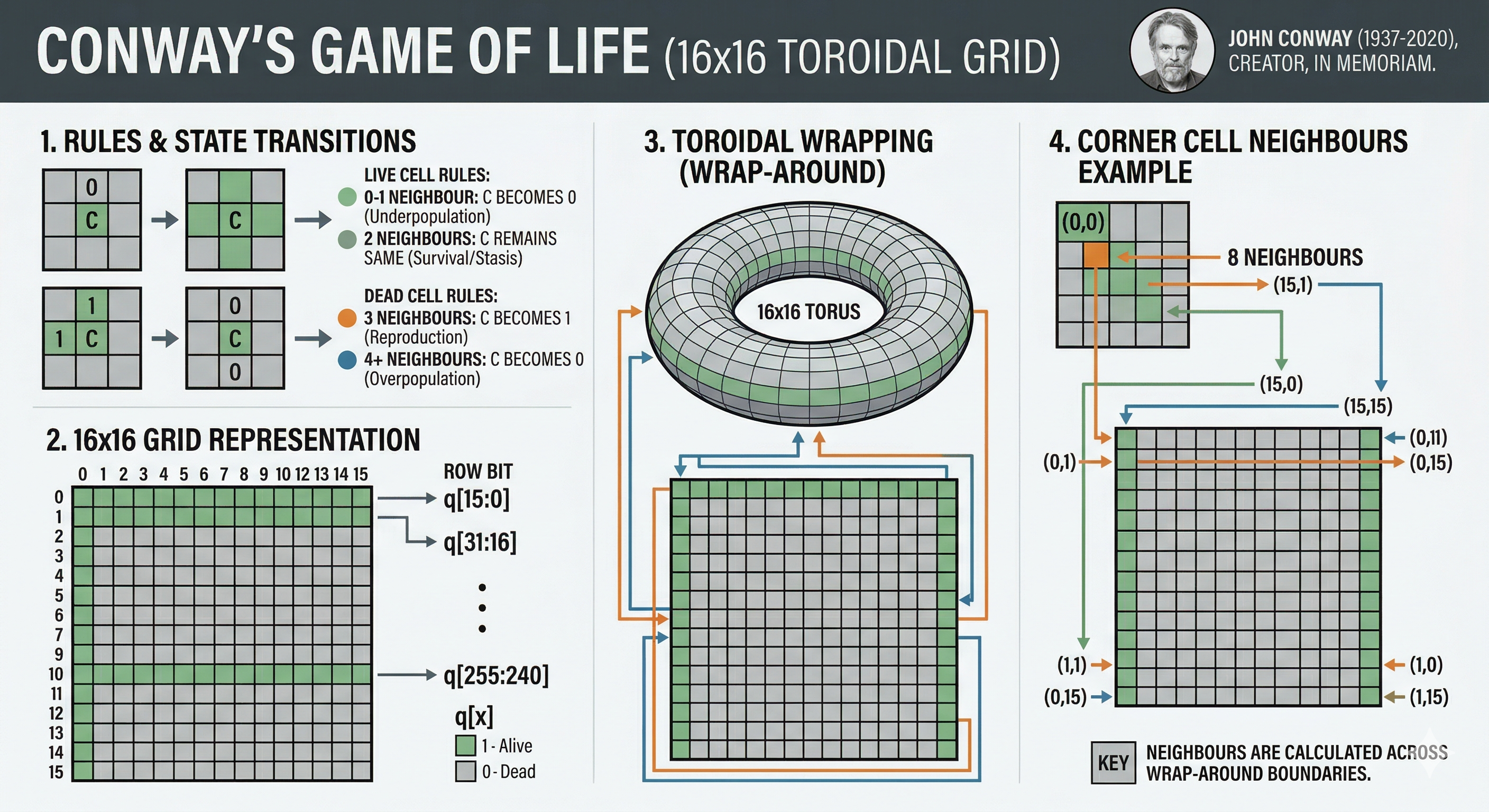
The “game” is played on a two-dimensional grid of cells, where each cell is either 1 (alive) or 0 (dead). At each time step, each cell changes state depending on how many neighbours it has:
- 0-1 neighbour: Cell becomes 0.
- 2 neighbours: Cell state does not change.
- 3 neighbours: Cell becomes 1.
- 4+ neighbours: Cell becomes 0.
The game is formulated for an infinite grid. In this circuit, we will use a 16x16 grid. To make things more interesting, we will use a 16x16 toroid, where the sides wrap around to the other side of the grid. For example, the corner cell (0,0) has 8 neighbours: (15,1), (15,0), (15,15), (0,1), (0,15), (1,1), (1,0), and (1,15). The 16x16 grid is represented by a length 256 vector, where each row of 16 cells is represented by a sub-vector: q[15:0] is row 0, q[31:16] is row 1, etc. (This tool accepts SystemVerilog, so you may use 2D vectors if you wish.)
- load: Loads data into q at the next clock edge, for loading initial state.
- q: The 16x16 current state of the game, updated every clock cycle.
The game state should advance by one timestep every clock cycle.
John Conway, mathematician and creator of the Game of Life cellular automaton, passed away from COVID-19 on April 11, 2020.
Hint
A test case that’s easily understandable and tests some boundary conditions is the blinker 256’h7. It is 3 cells in row 0 columns 0-2. It oscillates between a row of 3 cells and a column of 3 cells (in column 1, rows 15, 0, and 1).
Explanation by GEMINI
🧑💻 Code Example
You can also view my Github repo to see the whole project files, include below source code. Brandon-git-hub/Open_EDA_Example - Conwaylife (HDLBits)
RTL Code
module top_module(
    input clk,
    input load,
    input [255:0] data,
    output [255:0] q
);

    reg [15:0] grid [15:0];
    reg [15:0] next_grid [15:0];

    // Map the 2D grid to the output vector q
    genvar r_out;
    generate
        for (r_out = 0; r_out < 16; r_out = r_out + 1) begin : output_assign
            assign q[r_out*16 +: 16] = grid[r_out];
        end
    endgenerate

    // Load initial state or update the grid on each clock cycle
    integer i;
    always @(posedge clk) begin
        if (load) begin
            for (i = 0; i < 16; i = i + 1) begin
                grid[i] <= data[i*16 +: 16];
            end
        end else begin
            for (i = 0; i < 16; i = i + 1) begin
                grid[i] <= next_grid[i];
            end
        end
    end

    integer r, c;
    integer r_up, r_dn, c_l, c_r;
    reg [3:0] neighbors;

    always @(*) begin
        for (r = 0; r < 16; r = r + 1) begin
            for (c = 0; c < 16; c = c + 1) begin

                // Calculate the indices of the 8 neighbors with wrap-around
                r_up = (r == 15) ? 0  : r + 1;
                r_dn = (r == 0)  ? 15 : r - 1;
                c_r  = (c == 15) ? 0  : c + 1;
                c_l  = (c == 0)  ? 15 : c - 1;

                // Count the number of live neighbors
                neighbors = grid[r_up][c_l] + grid[r_up][c] + grid[r_up][c_r] +
                            grid[r][c_l]                    + grid[r][c_r]    +
                            grid[r_dn][c_l] + grid[r_dn][c] + grid[r_dn][c_r];

                case (neighbors)
                    4'd2:    next_grid[r][c] = grid[r][c]; // 2 neighbors:remain unchanged
                    4'd3:    next_grid[r][c] = 1'b1;       // 3 neighbors:become alive
                    default: next_grid[r][c] = 1'b0;       // 0-1 or 4+ neighbors:become dead
                endcase
            end
        end
    end

endmodule
Testbench Code
`timescale 1ns/1ps
module tb_top_module;
// Inputs
reg clk;
reg load;
reg [255:0] data;
// Outputs
wire [255:0] q;
// Instantiate the DUT (Device Under Test)
top_module dut (
.clk(clk),
.load(load),
.data(data),
.q(q)
);
initial begin
clk = 0;
forever #5 clk = ~clk; // 10ns period
end
initial begin
$dumpfile("tb_top_module.vcd");
$dumpvars(0, tb_top_module);
// Initialize Inputs
load = 0;
data = 'd0;
// Wait for global reset or startup
@(posedge clk);
load <= 1;
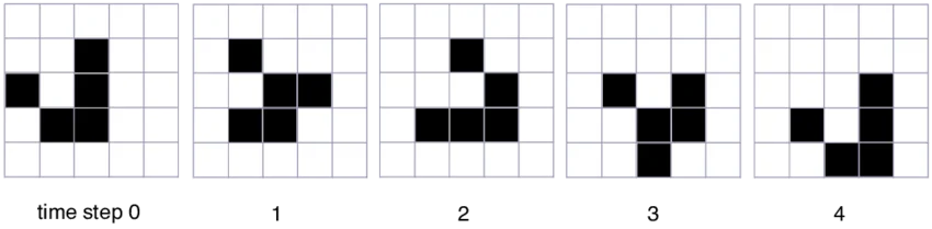
// Data for a Glider pattern
// (1,2), (2,3), (3,1), (3,2), (3,3)
data <= (256'b1 << (1*16 + 2)) |
(256'b1 << (2*16 + 3)) |
(256'b1 << (3*16 + 1)) |
(256'b1 << (3*16 + 2)) |
(256'b1 << (3*16 + 3));
@(posedge clk);
load <= 0;
// Run for some cycles
repeat (100) @(posedge clk);
$display("Simulation finished.");
$finish;
end
endmodule
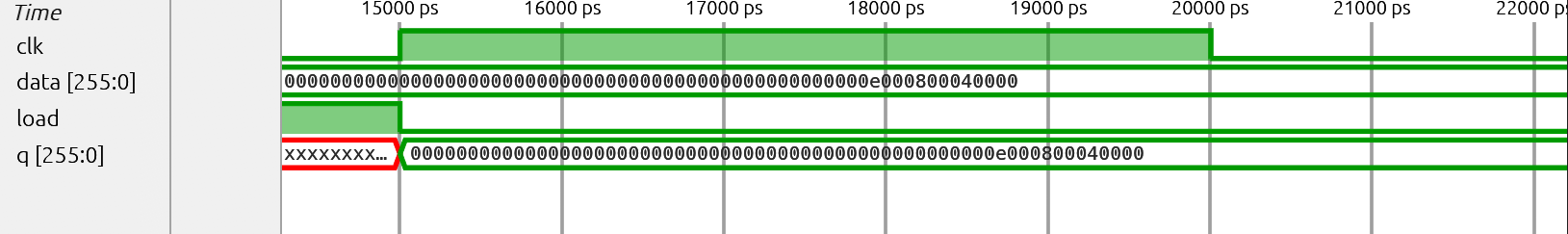
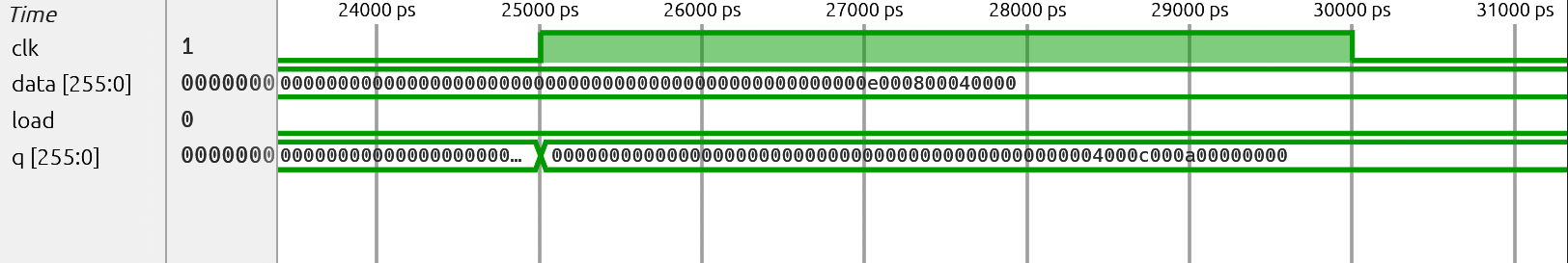
🔬 Results
Simulation Waveform
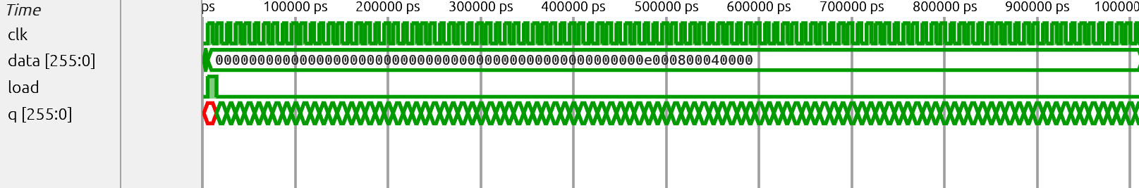
The initial pattern is like the middle one in the below image.